tripletTools Overview • tripletTools

Introduction

This package is designed to help analyze and visualize results from triadic comparisons (or triplet tasks), which are used to characterize the structure of mental representations. In a triplet task, a participant sees a referent item and two option items, and must decide which option is most similar to the referent. From many such judgments across many items and participants, one can compute a similarity embedding: a low-dimensional coordinate space in which items that are frequently judged as similar are placed nearby.

tripletTools does not collect data or compute embeddings — those steps occur outside R. Instead it provides tools for:

Loading triplet and embedding data files
Assessing participant data quality
Measuring inter-subject agreement on shared trials
Visualizing embeddings
Evaluating how well an embedding predicts held-out judgments
Quantifying individual differences in representation
Clustering participants by representational similarity

This vignette illustrates each of these steps using the example dataset included with the package.

library(tripletTools)

The example dataset

The package includes objects from a triplet study on 32 icon images of faces and buildings. The icons varied in category (face/building), time of day (day/night), and additional features (gender and race for faces; size and kind for buildings). Six participants each judged approximately 230 triplets online.

Object	Description
`icon_triplets`	Named list of 6 data frames, one per participant, containing trial-by-trial judgments
`icon_emb_ind`	Named list of 6 matrices, one per participant, containing 3-D embedding coordinates
`icon_emb_group`	Single data frame containing a 3-D group embedding
`icon_pics`	Named list of 32 PNG images, one per stimulus icon

Triplet data

Each element of icon_triplets is one participant’s trial data:

head(icon_triplets[[1]])
#>   head winner loser worker_id   rt Center  Left Right Answer  sampleAlg
#> 1   29     24    19  3n7ggxph 3096  pnhns pncnb pdcos  pncnb     random
#> 2   14      0    24  3n7ggxph 1100  fnmyb fdfob pncnb  fdfob     random
#> 3   30     19    24  3n7ggxph 2616  pnhob pncnb pdcos  pdcos     random
#> 4   17     12    13  3n7ggxph 2629  pdcns fnmow fnmob  fnmob validation
#> 5   29      9     8  3n7ggxph 2011  pnhns fnfow fnfob  fnfow     random
#> 6   25     23    12  3n7ggxph 1498  pncns fnmob pdhos  pdhos     random
#>   sampleSet
#> 1     train
#> 2     train
#> 3     train
#> 4     train
#> 5     train
#> 6     train

The key columns are Center (the referent item), Left and Right (the two options), Answer (the participant’s choice), sampleAlg (how the trial was sampled: random, check, or validation), and sampleSet (whether the trial was used to fit the embedding — train — or held out for testing — test).

Embedding data

Each element of icon_emb_ind is a 32-row matrix of 3-D embedding coordinates, with row names equal to stimulus names:

head(icon_emb_ind[[1]])
#>           dim_0     dim_1      dim_2
#> fdfob 0.6411938 0.9710717 -0.9336048
#> fdfow 0.5504593 0.9558654 -0.9130039
#> fdfyb 0.2907846 0.6866032 -0.6360701
#> fdfyw 0.5820549 0.9266087 -0.8992642
#> fdmob 0.5776460 1.0081034 -0.8230091
#> fdmow 0.7911357 0.4666237 -0.4759873

Data quality assessment

Before analyzing results it is good practice to check whether participants engaged with the task. get.participant.summary produces a per-participant summary including the number of trials completed, mean accuracy on check trials (easy triplets with an obvious answer used as an attention check), and mean log response time.

psummary <- get.participant.summary(icon_triplets, mintrial = 230)
head(psummary)
#>   tripfile worker_id ndat       lrt cacc keep
#> 1 3n7ggxph  3n7ggxph  230 0.4961625    1 TRUE
#> 2 b5wma4no  b5wma4no  230 0.9026607    1 TRUE
#> 3 d8mmm1qn  d8mmm1qn  230 0.5051381    1 TRUE
#> 4 jn7bbjc0  jn7bbjc0  230 0.6958144    1 TRUE
#> 5 pbby694o  pbby694o  230 0.6679493    1 TRUE
#> 6 sc2xbd6w  sc2xbd6w  230 0.6507582    1 TRUE

The output includes a keep column flagging participants who fall below the specified thresholds (the specified minimum number of trials, check-trial accuracy ≥ 0.80, mean log RT > 0). Participants failing these criteria should be reviewed before including their data in downstream analyses.

Inter-subject agreement on validation trials

A subset of trials — the validation trials — are drawn from a fixed pool shared across all participants, meaning the same triplets appear in multiple participants’ datasets. This allows us to measure inter-subject consistency: for each validation triplet we identify the majority vote (the option chosen by most participants who saw it) and the proportion of participants who agreed with that majority.

make.vmat computes this from the full triplet list:

vmat <- make.vmat(icon_triplets)

# One row per unique validation triplet
head(vmat$majority)
#>             triplet majority pmaj
#> 1 fdfow_fnmyb_pdhos    fnmyb  1.0
#> 2 fdmob_fdfow_pnhob    fdfow  1.0
#> 3 fdmob_fdmow_fdmyb    fdmyb  0.8
#> 4 fdmob_fnmob_pdcos    fnmob  1.0
#> 5 fdmow_fdmyw_fnfyw    fdmyw  1.0
#> 6 fdmow_fnfyw_pncnb    fnfyw  1.0

The pmaj column shows the proportion of participants who agreed with the majority choice. Values near 1.0 indicate near-universal agreement; values near 0.5 indicate a closely split decision.

hist(vmat$majority$pmaj,
     breaks = 10,
     main   = "Inter-subject agreement on validation trials",
     xlab   = "Proportion agreeing with majority vote",
     col    = "steelblue", border = "white")
abline(v = 0.5, lty = 2, col = "red")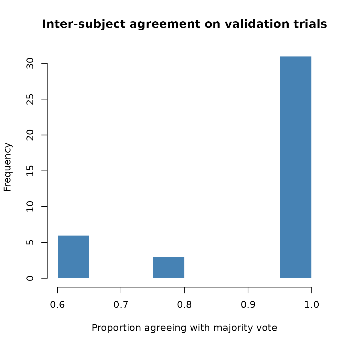

Distribution of inter-subject agreement on validation trials.

The bysbj element is a participant × triplet matrix recording whether each participant agreed with the majority vote (1), disagreed (0), or did not see the triplet (NA). The mean across triplets gives each participant’s overall agreement rate:

barplot(rowMeans(vmat$bysbj, na.rm = TRUE), 
        beside = T, 
        ylim = c(0, 1.0),
        xlab = "Participant",
        ylab = "Agreement",
        cex.names = 0.5,
        las=2)
box()
abline(h = 0.5, lty = 2)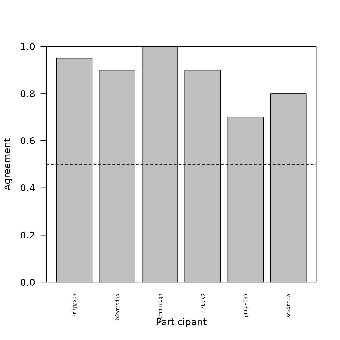

Participants can vary quite a bit as to how well they agree with the majority vote, indicating potential individual differences in how people view these stimuli.

Visualizing a 2-D embedding

plot_pics plots images as points in a scatterplot, positioned at their embedding coordinates. This gives an immediate visual impression of how the faces are organized in the learned similarity space.

emb1 <- icon_emb_ind[[1]]

plot_pics(emb1[,1:2], icon_pics,
          psize = 0.04,
          xlab  = "Dimension 1",
          ylab  = "Dimension 2",
          main  = "Embedding – participant 1")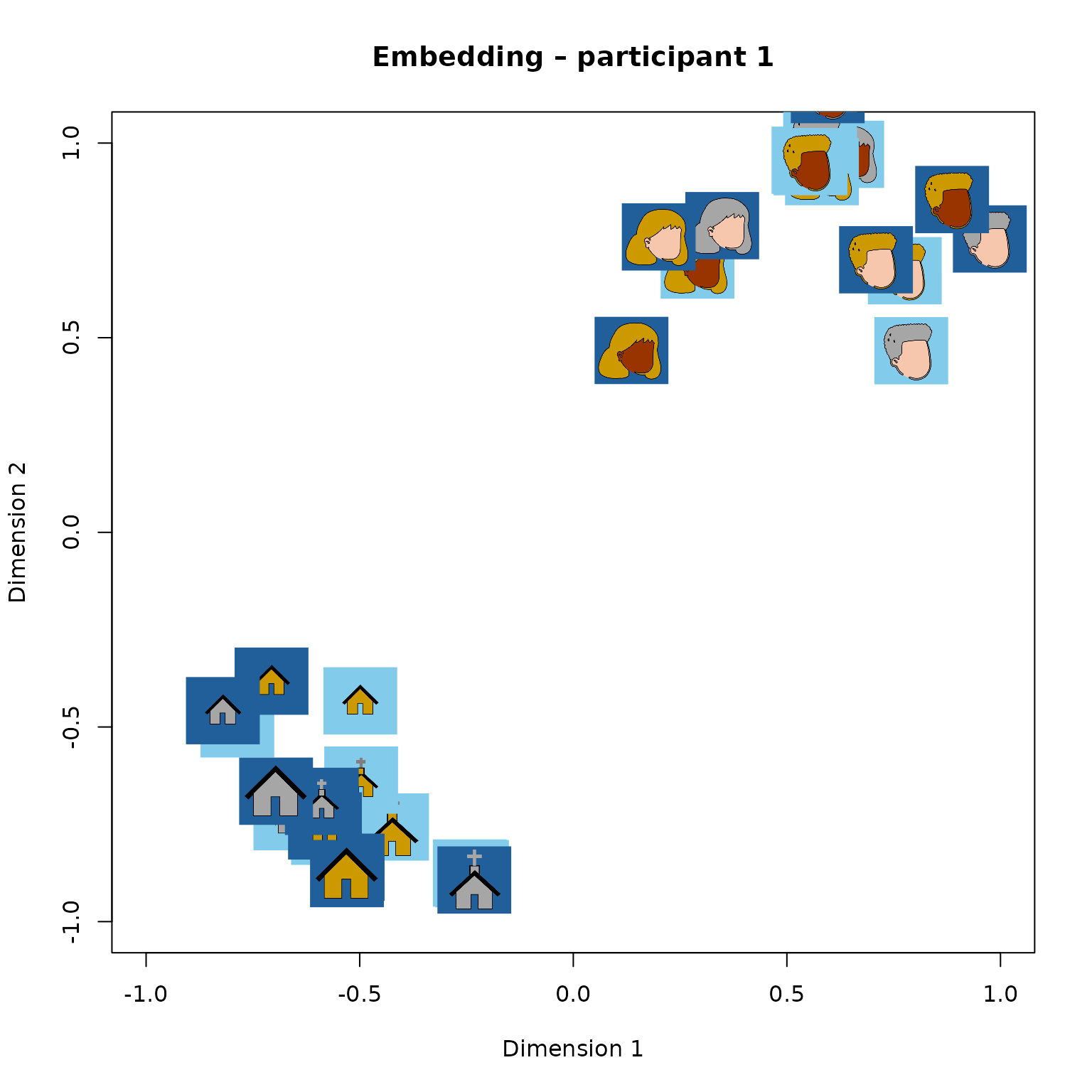

3-D embedding for participant 1, with icon images as points (first two dimensions shown).

Icons that appear close together were frequently judged as similar to one another by this participant.

Evaluating embedding quality: hold-out prediction accuracy

After computing an embedding we want to know how well it captures the participant’s actual judgments. For each held-out (test) triplet we can ask: does the embedding correctly predict which option the participant chose? The predicted choice is whichever option is closer to the referent in the embedding space.

get.hoacc returns the proportion of held-out trials for which the embedding’s prediction matches the participant’s answer:

acc1 <- get.hoacc(icon_emb_ind[[1]], icon_triplets[[1]])
cat("Hold-out prediction accuracy (participant 1):", round(acc1, 3), "\n")
#> Hold-out prediction accuracy (participant 1): 0.688

Chance performance is 0.50. Values above approximately 0.60 are generally considered reasonable for a 2-D embedding.

test.model returns trial-level predictions, making it easy to inspect specific errors or compute accuracy on any subset of trials:

result     <- test.model(icon_emb_ind[[1]], icon_triplets[[1]])
test_rows  <- result$sampleSet == "test"
mean(result$ModPred[test_rows] == result$Answer[test_rows], na.rm=TRUE)
#> [1] 0.6875

Prediction strength

model.strength computes, for each triplet, how decisively the embedding favors one option over the other. The metric is max(d1, d2) / (d1 + d2), where d1 and d2 are the distances from the referent to each option. It ranges from 0.5 (options equidistant from the referent) to 1.0 (one option far closer than the other).

If the embedding is well-calibrated, trials where it is most confident should also be the trials where participants agree most strongly. We can test this using the validation trials, for which we have an inter-subject agreement measure. NOTE: typically one would evaluate this for a group embedding, since validation statistics are computed across the whole group. Here we illustrate using the individual embedding from Participant 1; see icon_emb_group for the group embedding of these stimuli:

# Validation trials for participant 1
vtrips <- subset(icon_triplets[[1]], sampleAlg == "validation")

# Prediction strength from participant 1's embedding
pstrength <- model.strength(icon_emb_ind[[1]], vtrips)

# Locate matching inter-subject agreement values
tnames  <- make.tripnames(vtrips)
maj_idx <- match(tnames, vmat$majority$triplet)
pmaj    <- vmat$majority$pmaj[maj_idx]

# Plot the relationship
plot(pstrength, pmaj,
     xlab = "Embedding prediction strength",
     ylab = "Inter-subject agreement",
     pch  = 16, col = rgb(0, 0, 0.8, 0.4),
     main = "Strength vs. inter-subject agreement")
abline(lm(pmaj ~ pstrength), col = "red")

text(.5, .96, paste("r =", round(cor(pstrength, pmaj, use = "complete.obs"), 3)), adj = 0)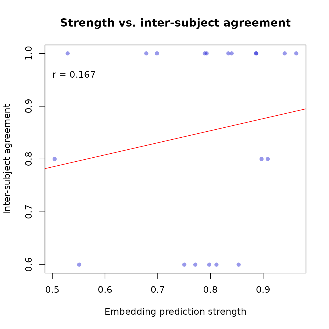

Embedding prediction strength vs. inter-subject agreement on validation trials.

A positive correlation indicates that the embedding correctly identifies which triplets have clearer, more consistent answers.

Individual differences: the prediction matrix

A central question in many triplet studies is whether participants differ reliably in their representations. The prediction matrix approach addresses this: we use each participant’s embedding to predict every other participant’s held-out judgments. If individual differences are real and systematic, a participant’s own embedding should predict their judgments better than another participant’s embedding does.

get.prediction.matrix computes this for all pairs:

pmat <- get.prediction.matrix(icon_emb_ind, icon_triplets)

The result is a 6 × 6 matrix. Entry [i, j] is the accuracy with which participant i’s embedding predicts participant j’s held-out judgments. The diagonal contains each participant’s self-prediction accuracy.

cat("Mean self-prediction accuracy:  ", round(mean(diag(pmat)), 3), "\n")
#> Mean self-prediction accuracy:   0.782
cat("Mean other-prediction accuracy: ", round(mean(pmat[row(pmat) != col(pmat)]), 3), "\n")
#> Mean other-prediction accuracy:  0.679

z.pred.mat converts each diagonal entry to a z-score relative to the other entries in its row, expressing how much better (or worse) a participant’s own embedding predicts their data compared to other participants’ embeddings:

zscores <- z.pred.mat(pmat)

cat("Mean z-score of self-prediction:", round(mean(zscores, na.rm = TRUE), 3), "\n")
#> Mean z-score of self-prediction: 1.022
cat("Proportion with positive z-score:", round(mean(zscores > 0, na.rm = TRUE), 3), "\n")
#> Proportion with positive z-score: 0.833

If z-scores are reliably positive across participants, this is evidence of meaningful individual differences in the representation of the stimulus set.

Representational distances between participants

get.rep.dist computes the pairwise procrustes distance between all pairs of embeddings. Two embeddings that can be brought into near-perfect alignment by rotation, scaling, and reflection have a low distance; embeddings that remain dissimilar after alignment have a high distance.

repdist <- get.rep.dist(icon_emb_ind)

We can cluster participants by their representational distances using standard hierarchical clustering:

#Compute hierarchical cluster tree:
hc     <- hclust(as.dist(repdist), method = "ward.D") 

#Cut tree into 2 clusters:
clusts <- cutree(hc, k = 2)

#Plot tree and highlight groups created by cutting:
plot(hc,
     labels = FALSE,
     main   = "Participant clustering by representational distance",
     xlab   = "", sub = "")
rect.hclust(hc, k = 2, border = c("tomato", "steelblue"))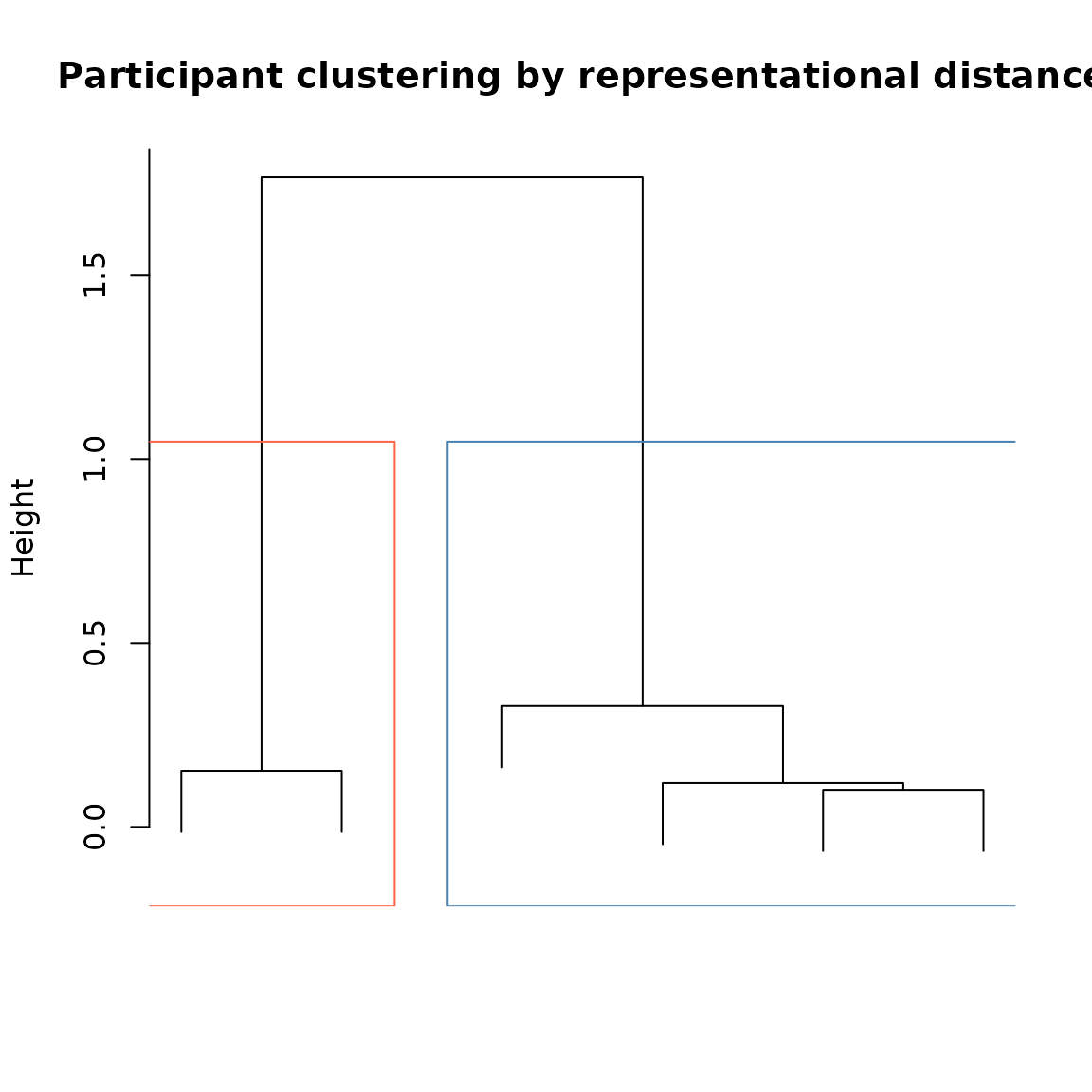

Participants clustered by pairwise representational distance.

Mean embedding per cluster

get.group.list.mean aligns all embeddings within each cluster and returns a mean embedding for each group:

mn_by_clust <- get.group.list.mean(icon_emb_ind, clusts)

Plotting each cluster’s mean embedding shows whether different groups of participants organized the icons in qualitatively different ways:


dmat <- mn_by_clust[[1]] #Copy data matrix
dmat <- dmat / max(abs(dmat)) #Max scaling

tripletTools::plot_pics(dmat, icon_pics, psize = 0.04,
          xlab = "Dimension 1", ylab = "Dimension 2",
          main = "Cluster 1 – mean embedding")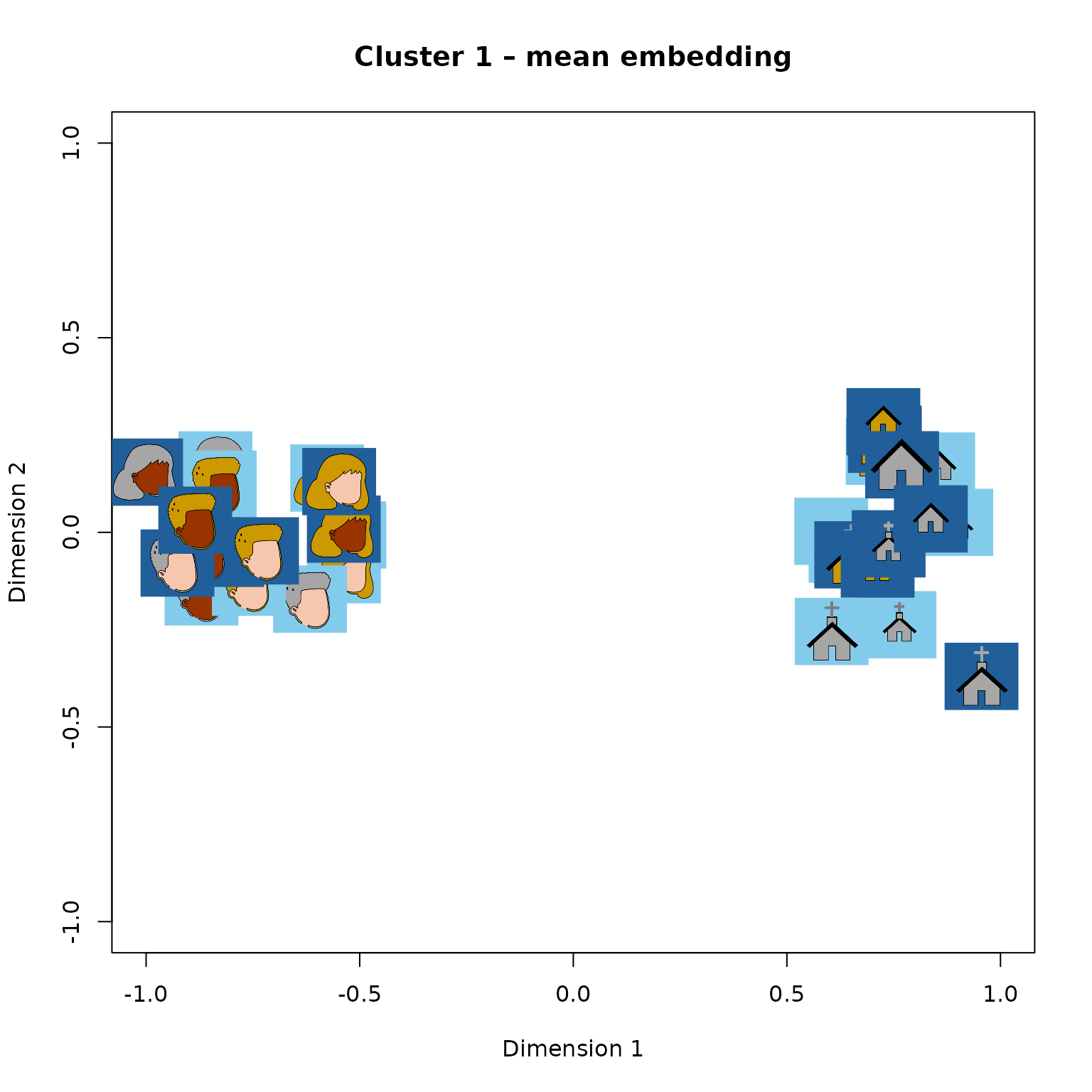

Mean embedding for cluster 1 (first two dimensions).

dmat <- mn_by_clust[[2]] #Copy data matrix
dmat <- dmat / max(abs(dmat)) #Max scaling

tripletTools::plot_pics(dmat, icon_pics, psize = 0.04,
          xlab = "Dimension 1", ylab = "Dimension 2",
          main = "Cluster 2 – mean embedding")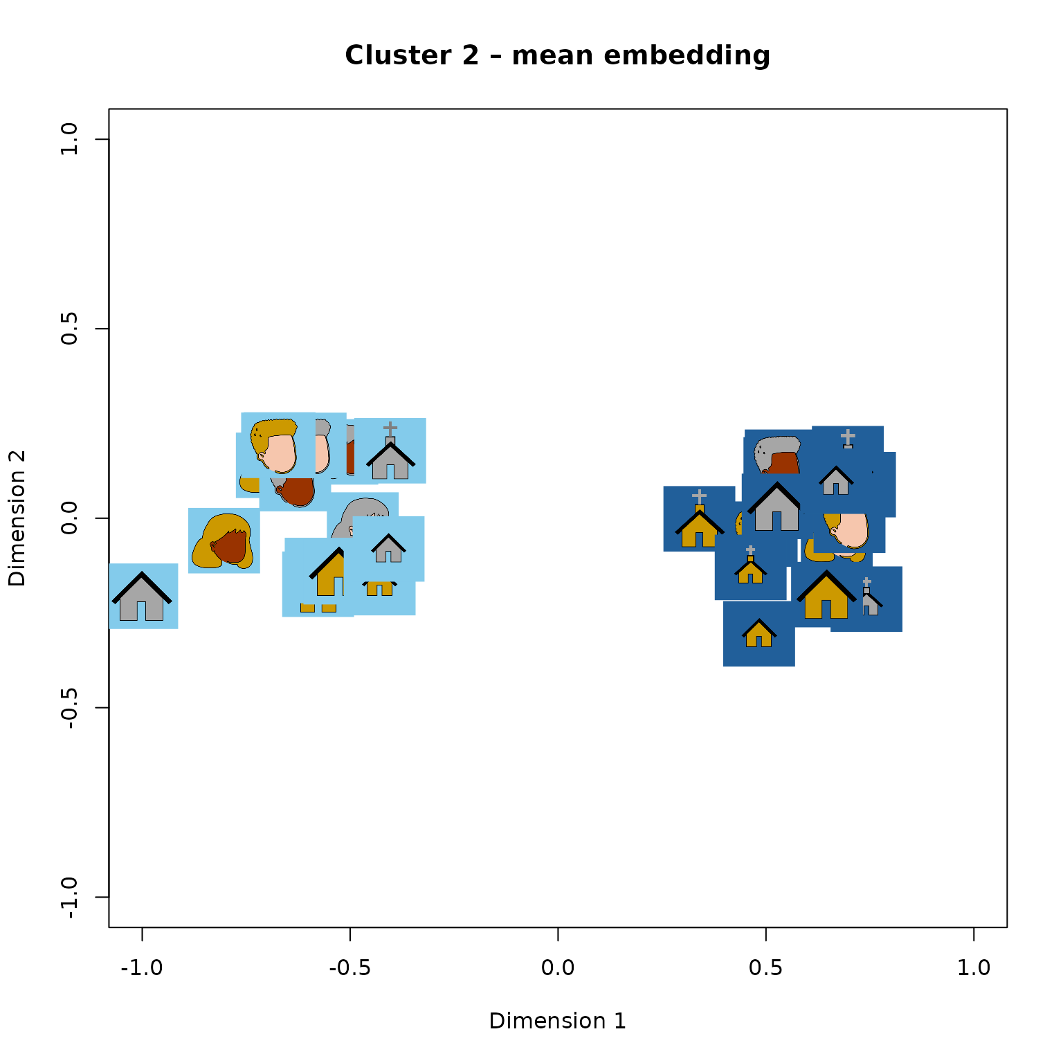

Mean embedding for cluster 2 (first two dimensions).

Prediction accuracy by cluster

If the clustering captures genuine individual differences, a participant’s held-out judgments should be better predicted by embeddings from within their cluster than by embeddings from other clusters. pacc.by.cluster tests this directly using the prediction matrix:

pbc <- pacc.by.cluster(pmat, clusts, samediff = TRUE)
head(pbc)
#>               self      same     other
#> 3n7ggxph 0.6875000 0.8050836 0.5735931
#> b5wma4no 0.8400000 0.7609392 0.5562771
#> d8mmm1qn 0.8461538 0.7062319 0.6038961
#> jn7bbjc0 0.7391304 0.7682692 0.5952381
#> pbby694o 0.8181818 0.8571429 0.6370255
#> sc2xbd6w 0.7619048 0.7575758 0.6082839

Each row is one participant. The three columns give prediction accuracy from (1) their own embedding, (2) the mean of their cluster-mates’ embeddings, and (3) the mean of participants outside their cluster.

round(colMeans(pbc), 3)
#>  self  same other 
#> 0.782 0.776 0.596

We can show the mean and 95% confidence interval of these values across participants as a ribbon plot:

plot_cis(pbc,
         xvals  = 1:3,
         main   = "Prediction accuracy by cluster membership",
         ylab   = "Hold-out prediction accuracy",
         xaxt   = "n",
         ylim   = c(0.5, 1.0))
axis(1, at = 1:3, labels = c("Self", "Same cluster", "Other cluster"))
abline(h = 0.5, lty = 2, col = "grey50")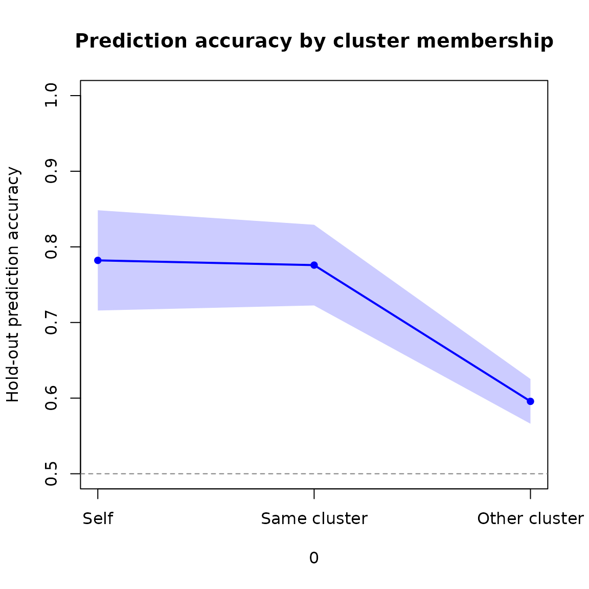

Hold-out prediction accuracy: self, same cluster, and other cluster.

A higher mean for “same cluster” than “other cluster” indicates that cluster membership captures something real about how participants differ in their representations.

Tree visualization with images as leaves

For a richer view of the similarity structure in one participant’s embedding, a hierarchical cluster tree with face images at the leaves can be more informative than a 2-D scatterplot — especially for higher-dimensional embeddings. get.tip.coords retrieves the tip coordinates of a phylogram plot, allowing plot_pics to place images at the correct positions. In this case we will visualize the hierarchical cluster plot of the single embedding computed from the full group of participants (icon_emb_group).

hc_emb <- hclust(dist(icon_emb_group[,1:3]), method = "ward.D2")
pt     <- ape::as.phylo(hc_emb)

plot(pt, type = "fan", show.tip.label = FALSE,
     main = "Icon similarity tree – group")

tip_coords <- get.tip.coords()
plot_pics(tip_coords, icon_pics, newplot = FALSE, psize = 0.04)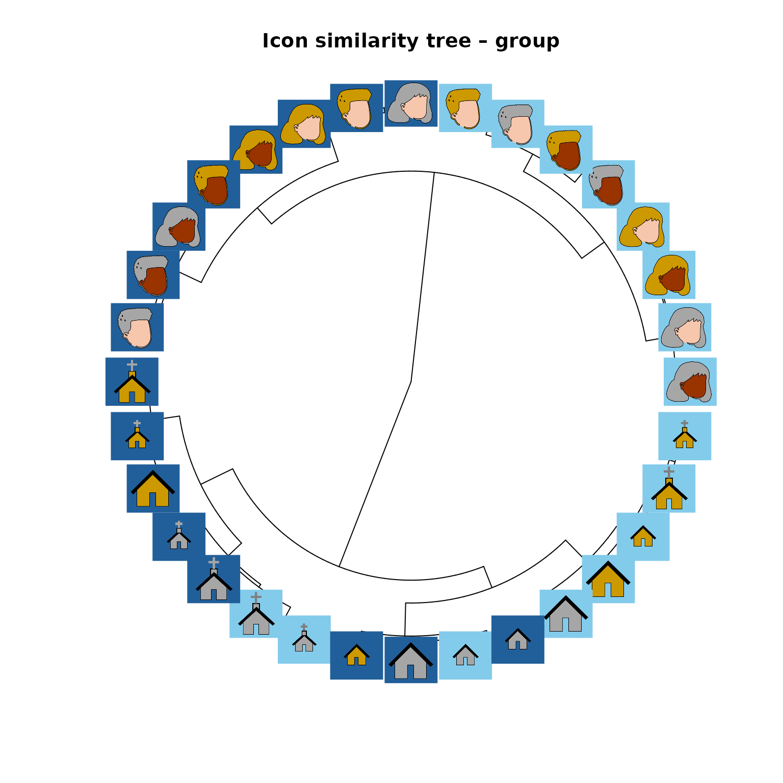

Similarity tree for participant 1, with icon images at the leaves.

Icons on nearby branches were judged as similar overall by the group.

Summary

The table below maps common analysis questions to the corresponding tripletTools functions:

Question	Function(s)
Did participants engage with the task?	`get.participant.summary`
How consistent are judgments across participants?	`make.vmat`
What does a participant’s embedding look like?	`plot_pics`
How well does the embedding predict held-out judgments?	`get.hoacc`, `test.model`
Does the embedding correctly rank triplet difficulty?	`model.strength`
Are individual differences in representation reliable?	`get.prediction.matrix`, `z.pred.mat`
How similar are two participants’ representations?	`get.rep.dist`
Are there subgroups with similar representations?	`get.rep.dist`, `get.group.list.mean`
Do cluster-mates predict each other’s data better?	`pacc.by.cluster`, `plot_cis`
How to show a full similarity tree with images?	`get.tip.coords`, `plot_pics`